This is the chapter Part I was preparing you for. We have data — the simulated laptop study of Section 7.6, 500 respondents making 4,000 choices — and we have every tool the estimation requires: the likelihood principle (Chapter 5), the stacked data representation (Chapter 4), and the numerical climber (Chapter 6). What remains is assembly, and assembly is where the details live: the exact form of the MNL log-likelihood, its gradient, a numerical trap and its escape, and the reporting and validation rituals that turn an optimizer’s output into research you can defend.
Start by loading the study — data and answer key — saved at the end of Chapter 7:
study <-readRDS("../data/laptop_study.rds")laptops <- study$databeta_true <- study$beta_trueX <-model.matrix(~ brand + ram + screen + price, data = laptops)[, -1]y <- laptops$choicetask_id <-cumsum(!duplicated(laptops[, c("id", "task")]))K <-ncol(X)c(rows =nrow(X), tasks =max(task_id), K = K)
 rows tasks     K
12000  4000     6
(The three lines rebuilding X, y, and task_id are build_choice_data() from Section 4.7 written out flat, so this chapter’s code is visible end to end.)
8.1 The MNL Log-Likelihood
The recipe of Chapter 5: the log-likelihood is the sum, over choice situations, of the log probability of the alternative actually chosen. With the switch-exponent device of Equation 5.3 generalized — let \(y_{ntj} = 1\) if alternative \(j\) was chosen in situation \((n,t)\) and 0 otherwise — the indicator encoding of Equation 7.2’s choice, and exactly the choice column of our long-format data — and the MNL probabilities of Equation 7.4 plugged in:
Because exactly one \(y_{ntj}\) per situation equals one, the inner sum simply selects the chosen row, and the whole expression collapses to something you can say in words: the log-likelihood is the sum, over choice situations, of the chosen alternative’s utility minus the log-sum of all alternatives’ exponentiated utilities.
Every term is a competition: how good was what they picked, against the log-sum measure of everything they could have picked. A candidate \(\boldsymbol{\beta}\) scores well when it makes chosen alternatives look systematically attractive relative to their own choice sets — not in absolute terms, which, per Section 7.5, the data could never reveal anyway.
8.2 Coding loglik_mnl()
Following our transparent-first discipline, the loop version walks tasks one at a time — for each, extract its rows, compute utilities, apply Equation 8.2:
loglik_mnl_loop <-function(beta, y, X, task_id) { ll <-0for (i inunique(task_id)) { rows <-which(task_id == i) V <- X[rows, , drop =FALSE] %*% beta ll <- ll + V[y[rows] ==1] -log(sum(exp(V))) }as.vector(ll)}
Readable, correct, and — as Chapter 9 will measure precisely — slow, because R pays interpreter overhead 4,000 times per likelihood evaluation, and the optimizer will request many evaluations. The vectorized version eliminates the loop using exactly the grouped-computation pattern rehearsed in Figure 7.1: compute all utilities in one matrix product, form all task-level log-sums with one rowsum() call, and broadcast them back to the rows by indexing:
loglik_mnl <-function(beta, y, X, task_id) { V <-as.vector(X %*% beta) # all NTJ utilities at once Vmax <-ave(V, task_id, FUN = max) # per-task max (stability; see below) eV <-exp(V - Vmax) denom <-rowsum(eV, task_id) # per-task sums, one grouped opsum( (V - Vmax -log(denom[task_id]))[y ==1] )}
Line by line against Equation 8.2: V is every \(V_{ntj}\); denom[task_id] puts each task’s \(\sum_{j'} e^{V_{ntj'}}\) next to each of its rows (indexing a vector by a group label — the broadcast idiom); the bracketed expression is every alternative’s log probability; and [y == 1] selects the chosen rows before summing. The Vmax lines are new, and they are the subject of the next section — ignore them for one moment and confirm the two implementations agree:
c(loop =loglik_mnl_loop(beta_true, y, X, task_id),vectorized =loglik_mnl(beta_true, y, X, task_id))
      loop vectorized
  -3774.99   -3774.99
Identical. One function, two implementations, same mathematics — keep the loop version as executable documentation, run the vectorized one.
8.3 The Log-Sum-Exp Trick
Now the Vmax business. The naive computation of \(\log \sum_{j'} e^{V_{j'}}\) evaluates exp() first, and exp() is an accident waiting to happen: exp(710) overflows to Inf, and exp(-746) underflows to 0. Our well-scaled laptop data keep utilities around \(\pm 3\), but recall the scaling discussion of Chapter 6: suppose a colleague hands you the same data with price in dollars, so the price coefficient should come out near \(-0.0012\). En route, the optimizer will surely try \(\boldsymbol{\beta}\) values like “\(-1.2\) on dollars,” producing utilities near \(-1800\):
V_bad <-c(-1795, -1801, -1808) # utilities under a mis-scaled candidatelog(sum(exp(V_bad))) # exp underflows to 0; log(0) = -Inf
[1] -Inf
An infinite log-likelihood poisons the optimizer — gradients become NaN, BFGS’s curvature updates corrupt, and the failure surfaces far from its cause. The escape is an identity: for any constant \(m\),
(factor \(e^m\) out of the sum). Choose \(m = \max_{j'} V_{j'}\): then every exponent is \(\le 0\), the largest term is exactly \(e^0 = 1\), and neither overflow nor total underflow can occur — the sum always lies in \([1, J]\):
m <-max(V_bad)m +log(sum(exp(V_bad - m))) # finite, correct
[1] -1794.998
That is what Vmax does in loglik_mnl(), computed per task by ave(). The cost is two cheap vectorized operations; the benefit is a likelihood that cannot blow up anywhere the optimizer wanders. Write it into every softmax-shaped computation you ever produce — including, later, the probability weights inside MSL (Chapter 12) and the Metropolis acceptance ratios of Chapter 15, both of which fail in exactly this way when coded naively.
8.4 The Analytic Gradient
BFGS will run on numerical gradients, but at \(2K\) extra likelihood evaluations per gradient (Equation 6.5 — two per parameter), analytic derivatives repay their derivation quickly — and for the MNL the derivation lands somewhere memorable. Differentiate one task’s contribution to Equation 8.2. The chosen alternative’s utility is linear, so it contributes \(\partial V_{ntj}/\partial \boldsymbol{\beta}= \mathbf{x}_{ntj}\). For the log-sum term, the chain rule gives \[\frac{\partial}{\partial \boldsymbol{\beta}} \log \sum_{j'} e^{V_{ntj'}} = \frac{\sum_{j'} e^{V_{ntj'}} \mathbf{x}_{ntj'}}{\sum_{j'} e^{V_{ntj'}}} = \sum_{j'} P_{ntj'} \, \mathbf{x}_{ntj'},\] the probability-weighted average of the task’s attribute rows — the model’s expected\(\mathbf{x}\). So each task contributes \(\mathbf{x}_{nt,\text{chosen}} - \sum_j P_{ntj} \mathbf{x}_{ntj}\): attributes of what they chose, minus attributes of what the model expected them to choose. Writing the chosen row with the indicators, \(\mathbf{x}_{nt,\text{chosen}} = \sum_j y_{ntj} \mathbf{x}_{ntj}\), and merging the two sums row-wise — stacking the indicators into \(\mathbf{y}\) and the probabilities into \(\mathbf{p}\), both length-\(NTJ\) vectors in the row order of \(\mathbf{X}\):
Identical in form to the binary logit scoreEquation 5.8: prediction errors times covariates, now with one error per alternative rather than per observation. At the MLE, the model’s predicted choice shares are exactly uncorrelated with every attribute. The implementation reuses the likelihood’s plumbing — and note this means the stability fix comes along free, since the probabilities are computed with the same shifted exponentials:
grad_mnl <-function(beta, y, X, task_id) { V <-as.vector(X %*% beta) Vmax <-ave(V, task_id, FUN = max) eV <-exp(V - Vmax) p <- eV /rowsum(eV, task_id)[task_id] # P_ntj for every rowas.vector(crossprod(X, y - p))}
Audit against the numerical gradient (num_grad() from Chapter 6), per standing policy — every analytic gradient gets checked:
num_grad <-function(fn, beta, h =1e-6, ...) { g <-numeric(length(beta))for (k inseq_along(beta)) { e <-replace(numeric(length(beta)), k, h) g[k] <- (fn(beta + e, ...) -fn(beta - e, ...)) / (2*h) } g}beta_test <-rep(0.1, K)rbind(analytic =grad_mnl(beta_test, y, X, task_id),numeric =num_grad(loglik_mnl, beta_test, y = y, X = X,task_id = task_id))
Six-decimal agreement. The algebra is certified; use the fast one.
8.5 Estimation
All pieces on the board — objective, gradient, climber. From a zero start (adequate here, per Chapter 6: the MNL log-likelihood is globally concave, so there is exactly one summit and no wrong basins):
fit <-optim(par =rep(0, K),fn = loglik_mnl,gr = grad_mnl,y = y, X = X, task_id = task_id,method ="BFGS",control =list(fnscale =-1),hessian =TRUE)fit$convergence
[1] 0
Converged. Standard errors from the curvature (Equation 5.10), and the full results table against the answer key:
Study this table for a moment; it is the first full-scale recovery in the book. Every estimate lands within a hair of its true value, every 95% interval covers the truth, and every \(|z|\) is enormous — with 4,000 choices, effects of this size are unmissable. The two memory coefficients illustrate invariance-in-action from Chapter 5: their difference (the marginal value of going from 16GB to 32GB, \(0.9 - 0.6 = 0.3\) in truth) is estimated by the difference of their estimates, 0.248. And the interpretation discipline of Section 7.5 applies: these are utilities on the arbitrary logit scale; the number a manager can use — dollars per attribute — waits for the WTP machinery of Chapter 21, which divides through by the price coefficient precisely to cancel the arbitrary scale.
8.6 Assessing Fit
An estimate without a fit assessment is a number without a context. Choice modelers lean on a small stable of measures, all built from log-likelihood values, all cheap now that estimation has run.
The null log-likelihood. The zero-parameter benchmark: every alternative equally likely, \(P = 1/J\) always. Because our unlabeled design has no ASCs, \(\boldsymbol{\beta}= \mathbf{0}\)is the null model,1 so \(\ell_0 = \sum_{n,t} \log(1/3) = -4000 \log 3\):
The likelihood-ratio test. Twice the log-likelihood gap, \(2(\ell_1 - \ell_0)\) — where \(\ell_1 = \ell(\hat{\boldsymbol{\beta}})\) is the maximized log-likelihood of the fit — is \(\chi^2\) with (here) 6 degrees of freedom under the null. Ours is 1246 — the null is not merely rejected, it is vaporized; unsurprising, since we simulated the alternatives to matter.
McFadden’s \(\rho^2\). The likelihood analogue of \(R^2\):
\[
\rho^2 = 1 - \frac{\ell_1}{\ell_0}
\tag{8.5}\]
rho2 <-1- fit$value / ll_nullround(rho2, 3)
[1] 0.142
Calibrate your expectations: \(\rho^2\) runs on a compressed scale, and values of 0.2–0.4 represent excellent fit for choice data Eggers et al. (2022). Ours, around 0.14, is exactly what a strong-but-noisy choice process yields — remember, the model’s own error term guarantees choices are not deterministic even with \(\boldsymbol{\beta}\) known perfectly.
Hit rate. The blunt-instrument check: how often is the modeled-most-probable alternative the chosen one?
V <-as.vector(X %*% fit$par)top <-ave(V, task_id, FUN = max) == Vmean(tapply(top & y ==1, task_id, any))
[1] 0.55125
Against a random-guess baseline of \(1/3\). Hit rates ignore probability calibration entirely (a 0.34 favorite and a 0.99 favorite count the same), so treat them as a communication device, not a model selection criterion.
AIC and BIC. For comparing non-nested specifications, penalized fit: \(\mathrm{AIC} = -2\ell + 2K\), \(\mathrm{BIC} = -2\ell + K \log(\text{observations})\). They earn their keep when the candidate models multiply — choosing the number of latent classes in Chapter 11 is where BIC becomes load-bearing for us.
8.7 Validation Against mlogit
Our estimator agrees with the truth, but “agrees with the truth on data we simulated” and “correctly implements maximum likelihood” are subtly different claims. The sharper test: an independent implementation, same data, same model — estimates should agree to numerical precision, not merely statistically. The mlogit package (Croissant 2020) is the R standard; feeding it requires only the index bookkeeping promised in Chapter 4 — a unique choice-situation id, a logical choice column, and dfidx()’s declaration of the panel structure:
(In mlogit’s three-part formula, alternative-varying attributes with generic coefficients occupy the first slot; the | 0 suppresses the ASCs that our unlabeled design must not have, per Section 4.5.) The confrontation:
Agreement to five decimals in coefficients, standard errors, and the log-likelihood itself. Two entirely separate codebases — ours, thirty transparent lines; theirs, a mature package — climbed to the same summit of the same surface. This is the validation ritual every estimator in this book will undergo where a reference implementation exists, and the divergence-hunting skills it builds transfer to the day one disagrees: coefficients matching but SEs differing (covariance estimator conventions), likelihoods differing by a constant (dropped combinatorial terms), estimates differing utterly (data-format misalignment — check the index construction first).
8.8 A Simulate-and-Recover Study
One recovery is an anecdote. The classical guarantees of Chapter 5 — consistency, asymptotic normality, honest standard errors — are statements about the distribution of \(\hat{\boldsymbol{\beta}}\) across repeated samples, and simulation lets us observe that distribution directly: rerun the entire pipeline — fresh study, fresh estimation — two hundred times and watch the estimator’s sampling behavior, not just one draw from it.
sim_and_fit <-function(N, T, J, beta) { df <-sim_mnl_data(N, T, J, beta) Xr <-model.matrix(~ brand + ram + screen + price, data = df)[, -1] tid <-cumsum(!duplicated(df[, c("id", "task")])) f <-optim(rep(0, length(beta)), loglik_mnl, gr = grad_mnl,y = df$choice, X = Xr, task_id = tid,method ="BFGS", control =list(fnscale =-1),hessian =TRUE)list(est = f$par, se =sqrt(diag(solve(-f$hessian))))}
               dell apple ram16 ram32 screen15  price
truth         0.500 1.000 0.600 0.900    0.300 -1.200
mean_estimate 0.498 0.997 0.596 0.895    0.302 -1.207
Bias indistinguishable from zero, coefficient by coefficient — consistency visibly at work at our sample size.
Is the sampling distribution normal, and are the standard errors honest? Overlay the 200 price-coefficient estimates with the normal density that the average estimated standard error implies:
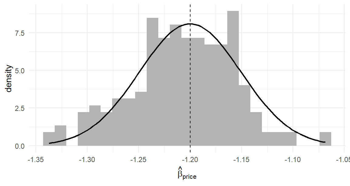
Figure 8.1: Sampling distribution of the price coefficient across 200 simulate-and-recover replications, with the normal density implied by the average estimated standard error. Asymptotic theory, audited and confirmed at 4,000 choice situations per replication.
The histogram is the actual sampling distribution; the curve is what the Hessian-based theory of Equation 5.10claims it should be. They match — which means the standard error printed in our results table is measuring exactly what it purports to measure. The numerical check: the empirical spread of estimates against the average claimed SE, all coefficients —
All within Monte Carlo noise of 0.95 (with 200 replications, the coverage estimate itself has an SE of about \(\sqrt{0.95 \times 0.05/200} \approx 0.015\)). The full classical package — centering, normality, honest uncertainty — verified by direct observation rather than trusted from a theorem. This replication audit is cheap insurance we will purchase again at moments of higher doubt: when simulation error enters the likelihood itself (Chapter 12) and when we need to compare frequentist and Bayesian machinery on equal footing (Chapter 17).
8.9 Key Learnings
The MNL log-likelihood is “chosen utility minus log-sum, summed over tasks” (Equation 8.2). Its vectorized implementation is three grouped operations — matrix product, rowsum(), broadcast-by-indexing — on the stacked data of Chapter 4.
exp() overflows and underflows; the log-sum-exp identity (Equation 8.3) with \(m = \max_{j'} V_{j'}\) makes the likelihood unconditionally safe, at negligible cost. Build it in by reflex, here and in every softmax you ever write.
The MNL score is \(\mathbf{X}'(\mathbf{y}- \mathbf{p})\) (Equation 8.4) — the binary logit’s “errors times covariates” form, unchanged. Derived, then audited against numerical differentiation, per standing policy.
Estimation recovered Equation 7.6 with tight, honest intervals; global concavity made the zero start safe. Fit was summarized by null log-likelihood, LR test, McFadden’s \(\rho^2\) (0.2–0.4 is excellent for choice data), hit rate, and AIC/BIC — all likelihood arithmetic.
Validation against mlogit agreed to five decimals in coefficients, SEs, and log-likelihood: two independent implementations, one summit. Every estimator in this book faces this ritual.
The 200-replication study observed the classical guarantees directly: unbiased centering, normal sampling distribution matching the claimed SEs, and 95% coverage. The MLE machine works — now we make it fast (Chapter 9) and point it at models that deserve the speed.
Croissant, Yves. 2020. “Estimation of Random Utility Models in R: The mlogit Package.”Journal of Statistical Software 95 (11): 1–41.
Eggers, Felix, Henrik Sattler, Thorsten Teichert, and Franziska Völckner. 2022. “Choice-Based Conjoint Analysis.” In Handbook of Market Research, edited by Christian Homburg, Martin Klarmann, and Arnd Vomberg, 781–819. Springer.
In a labeled design, the customary null keeps the ASCs (market shares) and drops everything else; the null is then the model’s fit with intercepts only, not \(N T \log(1/J)\). Know which null a reported statistic uses before comparing across papers.↩︎